CODE:
At Devise Foundation, we’re pioneering ConsciousLeaf—a 5D computational marvel that redefines precision and power, without the clutter of ML or quantum hype. Registered under the Indian Trust Act, our mission is to forge life-saving medicines and universal harmony through In silico innovation. We seek philanthropic partners passionate about next-level computing—systems that think beyond silicon.
Thursday, March 6, 2025
GNN ML Model code with optuna tuning for 6 SMILES and plot code
Friday, February 28, 2025
Predicted Toxicity: Curcumin vs Methylene Blue (MB)
CODE:
#CURCUMIN TOXICITY DATA
toxicity_predictions = {
'Hepatotoxicity': 0.69,
'Neurotoxicity': 0.87,
'Nephrotoxicity': 0.90,
'Respiratory toxicity': 0.98,
'Cardiotoxicity': 0.77,
'Immunotoxicity': 0.96,
'Ecotoxicity': 0.73
}
toxicity_types = list(toxicity_predictions.keys())
toxicity_probabilities = list(toxicity_predictions.values())
mb_toxicity_predictions = {
'Hepatotoxicity': 0.875, # Human Hepatotoxicity from ADMET
'Neurotoxicity': 0.911, # Drug-induced
'Nephrotoxicity': 0.878, # Drug-induced Nephrotoxicity from ADMET
'Respiratory toxicity': 0.436, # Respiratory from ADMET
'Cardiotoxicity': 0.77, # Assumed same as Curcumin
'Immunotoxicity': 0.098, # R
'Ecotoxicity': 0.0 # Adding Ecotoxicity for Methylene Blue, assuming 0 if no data
}
# Ensure the keys are identical to the Curcumin toxicity data
toxicity_types_mb = list(mb_toxicity_predictions.keys())
toxicity_probabilities_mb = list(mb_toxicity_predictions.values())
# Set the width of the bars
bar_width = 0.35
# Set the positions of the bars on the x-axis
r1 = np.arange(len(toxicity_types))
r2 = [x + bar_width for x in r1]
# Plotting the Toxicity Prediction
plt.figure(figsize=(12, 8))
# Make the plot for the toxicity prediction
plt.bar(r1, toxicity_probabilities, color='blue', width=bar_width, edgecolor='grey',
label='Curcumin')
plt.bar(r2, toxicity_probabilities_mb, color='green', width=bar_width, edgecolor='grey', label='Methylene Blue (MB)')
# General layout
plt.xlabel('Toxicity Type', fontsize=12)
plt.ylabel('Probability', fontsize=12)
plt.title('Predicted Toxicity: Curcumin vs Methylene Blue (MB)', fontsize=14)
plt.xticks([r + bar_width/2 for r in range(len(toxicity_types))], toxicity_types, rotation=45, ha='right', fontsize=10)
plt.ylim(0, 1.1) # Set y-axis limit from 0 to 1
plt.legend()
plt.tight_layout()
plt.savefig('toxicity_comparison_plot.png') # Save the plot as a file
plt.show()
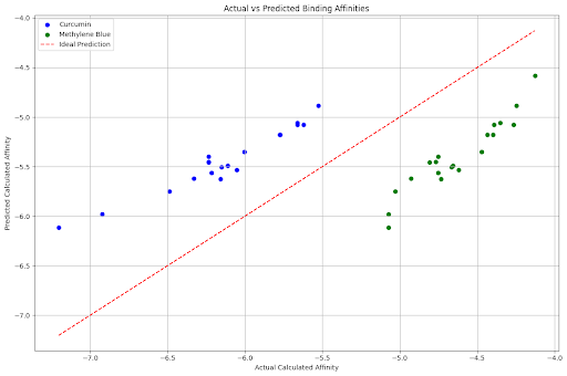
Actual vs Predicted Binding Affinity for Curcumin and Methylene Blue with TP53
CODE:
import pandas as pd
import json
from sklearn.model_selection import train_test_split
from sklearn.ensemble import RandomForestRegressor
from sklearn.metrics import mean_squared_error, r2_score
import matplotlib.pyplot as plt
import optuna
import numpy as np # Import numpy
# Debugging: Start script execution
print("Starting script execution...")
# 1. Data Loading and Preparation
print("Loading data...")
curcumin_data = {
'Model': list(range(1, 20)), # Model number (1 to 19)
'Calculated_affinity': [-7.204, -6.922, -6.488, -6.332, -6.236, -6.235, -6.234, -6.216, -6.159, -6.151,
-6.111, -6.052, -6.004, -5.777, -5.773, -5.663, -5.662, -5.622, -5.526]
}
curcumin_df = pd.DataFrame(curcumin_data)
curcumin_df['Molecule'] = 'Curcumin'
# Methylene Blue Binding Affinity Data (Revised)
binding_affinity_json = """
[
{"Model": 1, "Calculated affinity (kcal/mol)": -5.074},
{"Model": 2, "Calculated affinity (kcal/mol)": -5.073},
{"Model": 3, "Calculated affinity (kcal/mol)": -5.031},
{"Model": 4, "Calculated affinity (kcal/mol)": -4.927},
{"Model": 5, "Calculated affinity (kcal/mol)": -4.807},
{"Model": 6, "Calculated affinity (kcal/mol)": -4.766},
{"Model": 7, "Calculated affinity (kcal/mol)": -4.753},
{"Model": 8, "Calculated affinity (kcal/mol)": -4.751},
{"Model": 9, "Calculated affinity (kcal/mol)": -4.735},
{"Model": 10, "Calculated affinity (kcal/mol)": -4.666},
{"Model": 11, "Calculated affinity (kcal/mol)": -4.656},
{"Model": 12, "Calculated affinity (kcal/mol)": -4.621},
{"Model": 13, "Calculated affinity (kcal/mol)": -4.472},
{"Model": 14, "Calculated affinity (kcal/mol)": -4.436},
{"Model": 15, "Calculated affinity (kcal/mol)": -4.399},
{"Model": 16, "Calculated affinity (kcal/mol)": -4.390},
{"Model": 17, "Calculated affinity (kcal/mol)": -4.351},
{"Model": 18, "Calculated affinity (kcal/mol)": -4.266},
{"Model": 19, "Calculated affinity (kcal/mol)": -4.245},
{"Model": 20, "Calculated affinity (kcal/mol)": -4.127}
]
"""
binding_affinity_data = json.loads(binding_affinity_json)
mb_df = pd.DataFrame(binding_affinity_data)
mb_df['Molecule'] = 'Methylene Blue'
mb_df.rename(columns={'Calculated affinity (kcal/mol)': 'Calculated_affinity'}, inplace=True)
combined_df = pd.concat([curcumin_df, mb_df], ignore_index=True)
# Debugging: Check combined dataset
print("Combined dataset:")
print(combined_df.head())
X = combined_df[['Model']]
y = combined_df['Calculated_affinity']
X_train, X_test, y_train, y_test = train_test_split(X, y, test_size=0.2, random_state=42)
# Debugging: Data split check
print(f"Training set size: {len(X_train)}, Test set size: {len(X_test)}")
# Define the objective function for Optuna
def objective(trial):
n_estimators = trial.suggest_int('n_estimators', 50, 200)
max_depth = trial.suggest_int('max_depth', 3, 15)
min_samples_split = trial.suggest_int('min_samples_split', 2, 10)
model = RandomForestRegressor(n_estimators=n_estimators,
max_depth=max_depth,
min_samples_split=min_samples_split,
random_state=42)
model.fit(X_train, y_train)
y_pred = model.predict(X_test)
mse = mean_squared_error(y_test, y_pred)
return mse
# Run Optuna optimization
study = optuna.create_study(direction='minimize')
study.optimize(objective, n_trials=50)
best_params = study.best_params
print(f"Best hyperparameters: {best_params}")
final_rf_model = RandomForestRegressor(**best_params)
final_rf_model.fit(X_train, y_train)
# Calculate performance metrics on the test set
y_pred_test = final_rf_model.predict(X_test)
mse_test = mean_squared_error(y_test, y_pred_test)
r2_test = r2_score(y_test, y_pred_test)
# Print performance metrics for the test set
print(f"Test Set Mean Squared Error (MSE): {mse_test:.4f}")
print(f"Test Set R² Score: {r2_test:.4f}")
# Make predictions on the entire dataset for plotting
combined_df['Predicted_affinity'] = final_rf_model.predict(combined_df[['Model']])
plt.figure(figsize=(12, 8))
plt.scatter(combined_df[combined_df['Molecule'] == 'Curcumin']['Calculated_affinity'],
combined_df[combined_df['Molecule'] == 'Curcumin']['Predicted_affinity'],
color='blue', label='Curcumin')
plt.scatter(combined_df[combined_df['Molecule'] == 'Methylene Blue']['Calculated_affinity'],
combined_df[combined_df['Molecule'] == 'Methylene Blue']['Predicted_affinity'],
color='green', label='Methylene Blue')
plt.plot([combined_df['Calculated_affinity'].min(), combined_df['Calculated_affinity'].max()],
[combined_df['Calculated_affinity'].min(), combined_df['Calculated_affinity'].max()],
linestyle='--', color='red', label='Ideal Prediction')
plt.xlabel('Actual Calculated Affinity')
plt.ylabel('Predicted Calculated Affinity')
plt.title('Actual vs Predicted Binding Affinities')
plt.legend()
plt.grid(True)
plt.tight_layout()
# Save and display plot
output_file = 'actual_vs_predicted_affinity_combined.png'
plt.savefig(output_file)
print(f"Plot saved as: {output_file}")
# Show the plot if running interactively
plt.show()
Thursday, February 27, 2025
DRUG EFFICACY, DOSE RESPONSE
CODE:
Advanced Brain-Glucose & Neuron Analysis
Advanced Brain-Glucose Analyzer 🧠 Advanced Brain-Glucose & Neuron Analysis Multi-pa...
-
Concept Notes on Piezoelectric Shock Effects on Cellular Components for Uniform Laboratory Outcomes These concept notes explore the potentia...
-
Module 1: Core Cognitive Framework (No External Data) The foundational module operating purely on internal algorithms without external senso...
-
Hello, I'm a food lover born in Paikpara, Kolkata. From 1957 to 1996, I grew up in the lanes of Paikpara, and now I live in Rahara. My...


