
CODE:
import pandas as pd
import json
from sklearn.model_selection import train_test_split
from sklearn.ensemble import RandomForestRegressor
from sklearn.metrics import mean_squared_error, r2_score
import matplotlib.pyplot as plt
import optuna
import numpy as np # Import numpy
# Debugging: Start script execution
print("Starting script execution...")
# 1. Data Loading and Preparation
print("Loading data...")
curcumin_data = {
'Model': list(range(1, 20)), # Model number (1 to 19)
'Calculated_affinity': [-7.204, -6.922, -6.488, -6.332, -6.236, -6.235, -6.234, -6.216, -6.159, -6.151,
-6.111, -6.052, -6.004, -5.777, -5.773, -5.663, -5.662, -5.622, -5.526]
}
curcumin_df = pd.DataFrame(curcumin_data)
curcumin_df['Molecule'] = 'Curcumin'
# Methylene Blue Binding Affinity Data (Revised)
binding_affinity_json = """
[
{"Model": 1, "Calculated affinity (kcal/mol)": -5.074},
{"Model": 2, "Calculated affinity (kcal/mol)": -5.073},
{"Model": 3, "Calculated affinity (kcal/mol)": -5.031},
{"Model": 4, "Calculated affinity (kcal/mol)": -4.927},
{"Model": 5, "Calculated affinity (kcal/mol)": -4.807},
{"Model": 6, "Calculated affinity (kcal/mol)": -4.766},
{"Model": 7, "Calculated affinity (kcal/mol)": -4.753},
{"Model": 8, "Calculated affinity (kcal/mol)": -4.751},
{"Model": 9, "Calculated affinity (kcal/mol)": -4.735},
{"Model": 10, "Calculated affinity (kcal/mol)": -4.666},
{"Model": 11, "Calculated affinity (kcal/mol)": -4.656},
{"Model": 12, "Calculated affinity (kcal/mol)": -4.621},
{"Model": 13, "Calculated affinity (kcal/mol)": -4.472},
{"Model": 14, "Calculated affinity (kcal/mol)": -4.436},
{"Model": 15, "Calculated affinity (kcal/mol)": -4.399},
{"Model": 16, "Calculated affinity (kcal/mol)": -4.390},
{"Model": 17, "Calculated affinity (kcal/mol)": -4.351},
{"Model": 18, "Calculated affinity (kcal/mol)": -4.266},
{"Model": 19, "Calculated affinity (kcal/mol)": -4.245},
{"Model": 20, "Calculated affinity (kcal/mol)": -4.127}
]
"""
binding_affinity_data = json.loads(binding_affinity_json)
mb_df = pd.DataFrame(binding_affinity_data)
mb_df['Molecule'] = 'Methylene Blue'
mb_df.rename(columns={'Calculated affinity (kcal/mol)': 'Calculated_affinity'}, inplace=True)
combined_df = pd.concat([curcumin_df, mb_df], ignore_index=True)
# Debugging: Check combined dataset
print("Combined dataset:")
print(combined_df.head())
X = combined_df[['Model']]
y = combined_df['Calculated_affinity']
X_train, X_test, y_train, y_test = train_test_split(X, y, test_size=0.2, random_state=42)
# Debugging: Data split check
print(f"Training set size: {len(X_train)}, Test set size: {len(X_test)}")
# Define the objective function for Optuna
def objective(trial):
n_estimators = trial.suggest_int('n_estimators', 50, 200)
max_depth = trial.suggest_int('max_depth', 3, 15)
min_samples_split = trial.suggest_int('min_samples_split', 2, 10)
model = RandomForestRegressor(n_estimators=n_estimators,
max_depth=max_depth,
min_samples_split=min_samples_split,
random_state=42)
model.fit(X_train, y_train)
y_pred = model.predict(X_test)
mse = mean_squared_error(y_test, y_pred)
return mse
# Run Optuna optimization
study = optuna.create_study(direction='minimize')
study.optimize(objective, n_trials=50)
best_params = study.best_params
print(f"Best hyperparameters: {best_params}")
final_rf_model = RandomForestRegressor(**best_params)
final_rf_model.fit(X_train, y_train)
# Calculate performance metrics on the test set
y_pred_test = final_rf_model.predict(X_test)
mse_test = mean_squared_error(y_test, y_pred_test)
r2_test = r2_score(y_test, y_pred_test)
# Print performance metrics for the test set
print(f"Test Set Mean Squared Error (MSE): {mse_test:.4f}")
print(f"Test Set R² Score: {r2_test:.4f}")
# Make predictions on the entire dataset for plotting
combined_df['Predicted_affinity'] = final_rf_model.predict(combined_df[['Model']])
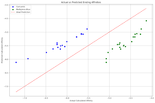
plt.figure(figsize=(12, 8))
plt.scatter(combined_df[combined_df['Molecule'] == 'Curcumin']['Calculated_affinity'],
combined_df[combined_df['Molecule'] == 'Curcumin']['Predicted_affinity'],
color='blue', label='Curcumin')
plt.scatter(combined_df[combined_df['Molecule'] == 'Methylene Blue']['Calculated_affinity'],
combined_df[combined_df['Molecule'] == 'Methylene Blue']['Predicted_affinity'],
color='green', label='Methylene Blue')
plt.plot([combined_df['Calculated_affinity'].min(), combined_df['Calculated_affinity'].max()],
[combined_df['Calculated_affinity'].min(), combined_df['Calculated_affinity'].max()],
linestyle='--', color='red', label='Ideal Prediction')
plt.xlabel('Actual Calculated Affinity')
plt.ylabel('Predicted Calculated Affinity')
plt.title('Actual vs Predicted Binding Affinities')
plt.legend()
plt.grid(True)
plt.tight_layout()
# Save and display plot
output_file = 'actual_vs_predicted_affinity_combined.png'
plt.savefig(output_file)
print(f"Plot saved as: {output_file}")
# Show the plot if running interactively
plt.show()


No comments:
Post a Comment